The goals / steps of this project are the following:
- Compute the camera calibration matrix and distortion coefficients given a set of chessboard images.
- Apply a distortion correction to raw images.
- Use color transforms, gradients, etc., to create a thresholded binary image.
- Apply a perspective transform to rectify binary image (“birds-eye view”).
- Detect lane pixels and fit to find the lane boundary.
- Determine the curvature of the lane and vehicle position with respect to center.
- Warp the detected lane boundaries back onto the original image.
- Output visual display of the lane boundaries and numerical estimation of lane curvature and vehicle position.
Here I will consider the rubric points individually and describe how I addressed each point in my implementation.
This writeup will describe the steps taken to find lane lines and challenges faced.
Camera Calibration
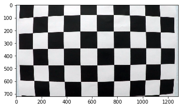
When images taken from camera lens, it involves lens distortion due to
varying angle of light in edge of lens. However by taking couple of sample
images we can get the conversion matrix / coefficients for removing the
distortion. First we will take couple of images of chess board or equivalent
and see how it is distorted. By as we know chess board will have squares
in it and distorted images skew the squares. We can use OpenCV
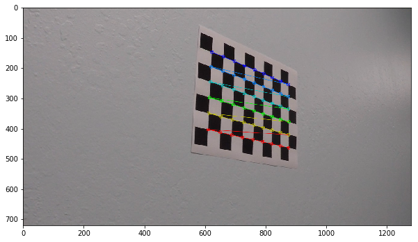
function findChessboardCorners to find the corners of chess board.
When we map those to our chess board coordinate system with calibrateCamera
I started with following image:
The code for this step is contained in the 3rd code cell of the IPython notebook located in “AdvancedLaneDetection.ipynb”
I start by preparing “object points”, which will be the (x, y, z) coordinates
of the chessboard corners in the world. Here I am assuming the chessboard
is fixed on the (x, y) plane at z=0, such that the object points are the
same for each calibration image. Thus, objp is just a replicated array
of coordinates, and objpoints will be appended with a copy of it every
time I successfully detect all chessboard corners in a test image. imgpoints
will be appended with the (x, y) pixel position of each of the corners in
the image plane with each successful chessboard detection.
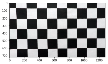
I then used the output objpoints and imgpoints to compute the camera
calibration and distortion coefficients using the cv2.calibrateCamera()
function. I applied this distortion correction to the test image using
the cv2.undistort() function and obtained this result:
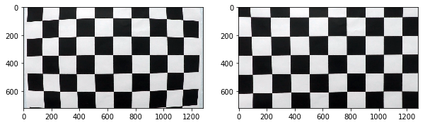
Here is both side by side for reference:
Pipeline (single image)
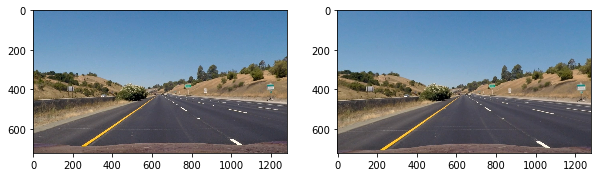
1. Provide an example of a distortion-corrected image.
To demonstrate this step, I will describe how I apply the distortion correction to one of the test images like this one:
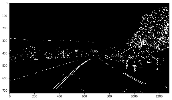
2. Transformation and binarized image
I used a combination of color in HLS and R channel threshold and gradient thresholds to generate a binary image (thresholding steps at lines # through # in the notebook). Here’s an example of my output for this step. (note: this is not actually from one of the test images)
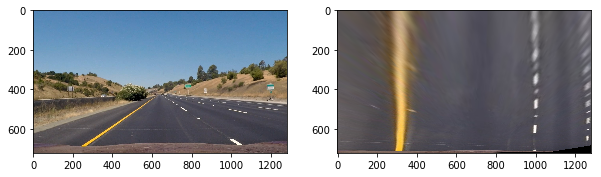
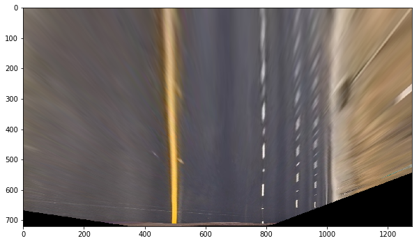
3. Now lets see same image transformed as if its viewed from top
The code for my perspective transform includes a function called warp() that takes as inputs an image (img), as well as source (src) and destination (dst) points. I chose the hardcode the source and destination points in the following manner:
def warp(img, M):
    img_size = (img.shape[1], img.shape[0])
    return cv2.warpPerspective(img, M, img_size, flags=cv2.INTER_LINEAR)
Following source and destination points were used by observing the image:
| Source | Destination |
|---|---|
| 244, 687 | 492, 687 |
| 1054, 679 | 790, 679 |
| 750, 490 | 790, 490 |
| 541, 489 | 492, 489 |
I verified that my perspective transform was working as expected by drawing the src and dst points onto a test
image and its warped counterpart to verify that the lines appear parallel in the warped image.
Belor is another possible transformation that I tried before, however this was covering more than our interested area so modified transformation mapping to pick the road lane.
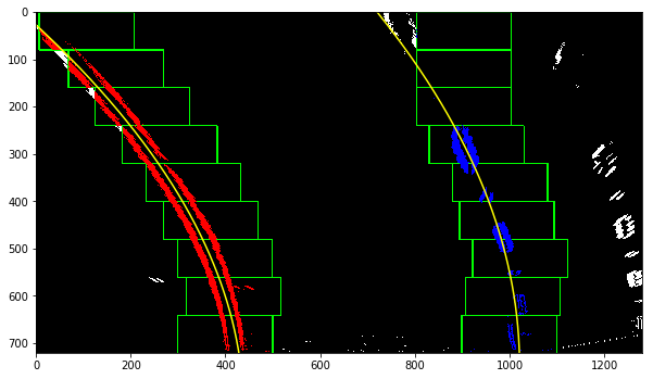
4. Polynomial fitting the lane pixels
In order to find the lane line I took botom portion of image and calculated histogram on binary image. Choosing max on left and right side gave position of lane line. From there a sliding window was used to fit the line.
5. Radius of curvature of road.
In order to compute the radius of curvature of the road aproximating the length of road in view as 50 meters and width of road lane as 3.5 meters. Our transformed road lane is measuring about 700 pixel wide and 720 pixel in run length.
ym_per_pix = 50/720.0 # meters per pixel in y dimension
xm_per_pix = 3.7/700.0 # meters per pixel in x dimension

left_fit_cr = np.polyfit(xy[0]*ym_per_pix, xy[1]*xm_per_pix, 2)
right_fit_cr = np.polyfit(xy[2]*ym_per_pix, xy[3]*xm_per_pix, 2)

y_eval = txbinary.shape[0]

left_curverad = ((1 + (2*left_fit_cr[0]*y_eval*ym_per_pix + left_fit_cr[1])**2)**1.5) / np.absolute(2*left_fit_cr[0])
right_curverad = ((1 + (2*right_fit_cr[0]*y_eval*ym_per_pix + right_fit_cr[1])**2)**1.5) / np.absolute(2*right_fit_cr[0])
# Now our radius of curvature is in meters
print(left_curverad, 'm', right_curverad, 'm')
To calculate the car position in lane, I used mapping pixel to meter. Difference between center of car from detected lane positions and center of camera will give the offset position.
def offset(txbinary, xy):
    xm_per_pix = 3.7/700.0
    return ((xy[1][0] + (xy[3][0] - xy[1][0] )/2) - txbinary.shape[1]/2 )* xm_per_pix
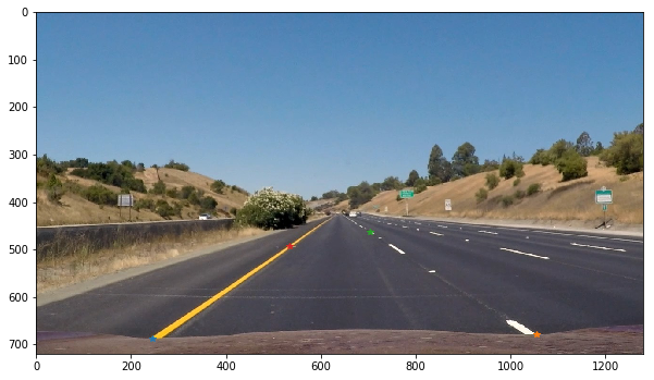
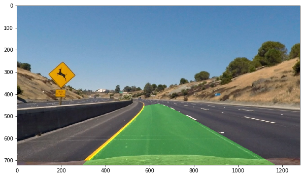
6. Provide an example image of your result plotted back down onto the road such that the lane area is identified clearly.
I implemented this step in the function plotThePath(). Here is an example of my result on a test image:
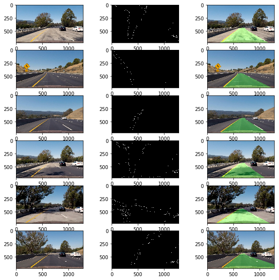
Pipeline (video)
1. Running above pipeline on image frame by frame on video taken while driving.
Here’s a Processed Video
Discussion
Here I’ll talk about the approach I took, what techniques I used, what worked and why, where the pipeline might fail and how I might improve it if I were going to pursue this project further.
In nutshell, pipeline consists of following steps
- fix lens distortion
- use color space with threshold to extract the lane lines
- Convert to binary using gradients on x and y
- transform the image as if its viewed by top
- Using window size of 100, 9 windows fit the line on image and find coefficient
Finally mark the lane boundaries on image.
Possible failures
Found problem in processing shadows, different colored pavement, in order to cover such scenarios I had to use S and Red channels
Processing is sensitive to other marking that may be found on road. Probably using last found line position and searching from there would solve this issue.
Potential improvements
Hold the state and write confidence score based on information that is available. For example left and right should run parallel if they vary in direction or curvature we can either reject or take weighted average.
Retain the lane position and start searching for same position in next frame, a sliding window would help in adjusting actual position.
Possibly use canny edge in lower portion to start window search, this may help in ignoring other signs on the road.